Surf-plotting scattered data in Matlab (or: Delaunay interpolation without a grid)
Matlab has a number of methods for interpolating data, both for data that is sampled on a regular grid and for data that is “scattered”, or randomly distributed.
Surface plotting
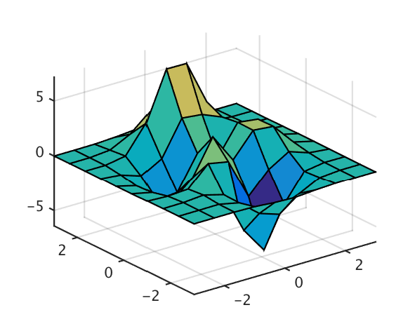
Plotting surfaces over grid points is easy using Matlab’s surf command, and interpolation of that data to get smoother plots is straightforward. For example,
[x,y,z] = peaks(10);
surf(x,y,z);
will plot:
Generally I recommend avoiding 3D plots, so in 2D (view(2)):
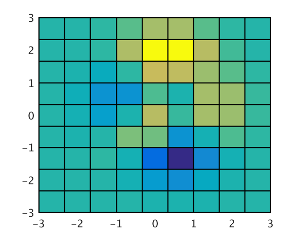
The variables x and y are 10x10 matrices defined by (the equivalent of) [x,y]=meshgrid(linspace(-3,3,10)), and z is the value at each point in (x,y) space.
If you have sampled data with non-uniform spacing, however, it’s not as obvious how to plot that data. In this case your data would be organised with x, y, and z as column vectors with each measurement per row. The structure of the surf command simply doesn’t handle data in this form, since the data isn’t organised in a way that allows adjacent points to be connected.
Matlab provides commands for analysing this data using Delaunay Triangulation, for which it also provides an analogue to surf. Here’s an example:
N = 15;
rng(13); % repeatable random values
x = randn(1,N); % X & Y coords
y = randn(1,N);
z = randn(1,N); % "value" at each coordinate
After a little digging, you’ll find that the easiest way to plot this data as a surface is:
trisurf(delaunay(x,y),x,y,z)
Seems slightly redundant, but easy enough.
Surf plots with coarse grids
The problem is that surface plots are poor at visualising data over coarse meshes, since it’s their corners which define the values. This can be seen in the following example, using peaks to plot a surface:
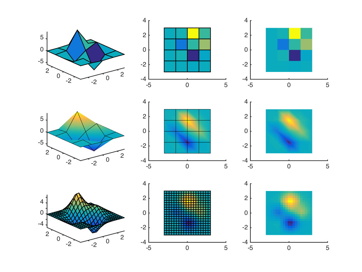
The first row shows plain surf. It can be seen that the colours of each “patch” don’t do a good job of representing their height (or “value”). In the second row, Matlab’s interpolating shader is used to “improve” this. It’s an improvement, but distortions are obvious where there are large changes in both directions. (Colours are smeared along diagonals, basically.)
Finally, in the third row an interpolation function is used to generate more data points. This is quite a coarse interpolation, but couldn’t go finer without the edges taking over in the 3D plot. The plot looks far more convincing. Gridded interpolation can be done in a number of ways; for this example I used
F = griddedInterpolant(x',y',z');
[x2,y2] = ndgrid(linspace(-3,3,20));
surf(x2,y2,F(x2,y2))
(The transpose being necessary from coordinates output from peaks. Good old Matlab.)
Surf plots with coarse scattered data
But what about scattered data? While Matlab does provide scatteredInterpolant, this form is only really convenient if you want to interpolate onto a regular grid. What if you just want to improve the look of your overly-coarse surface plot? Here’s the example using trisurf described above, with and without interpolated shading (shading interp):
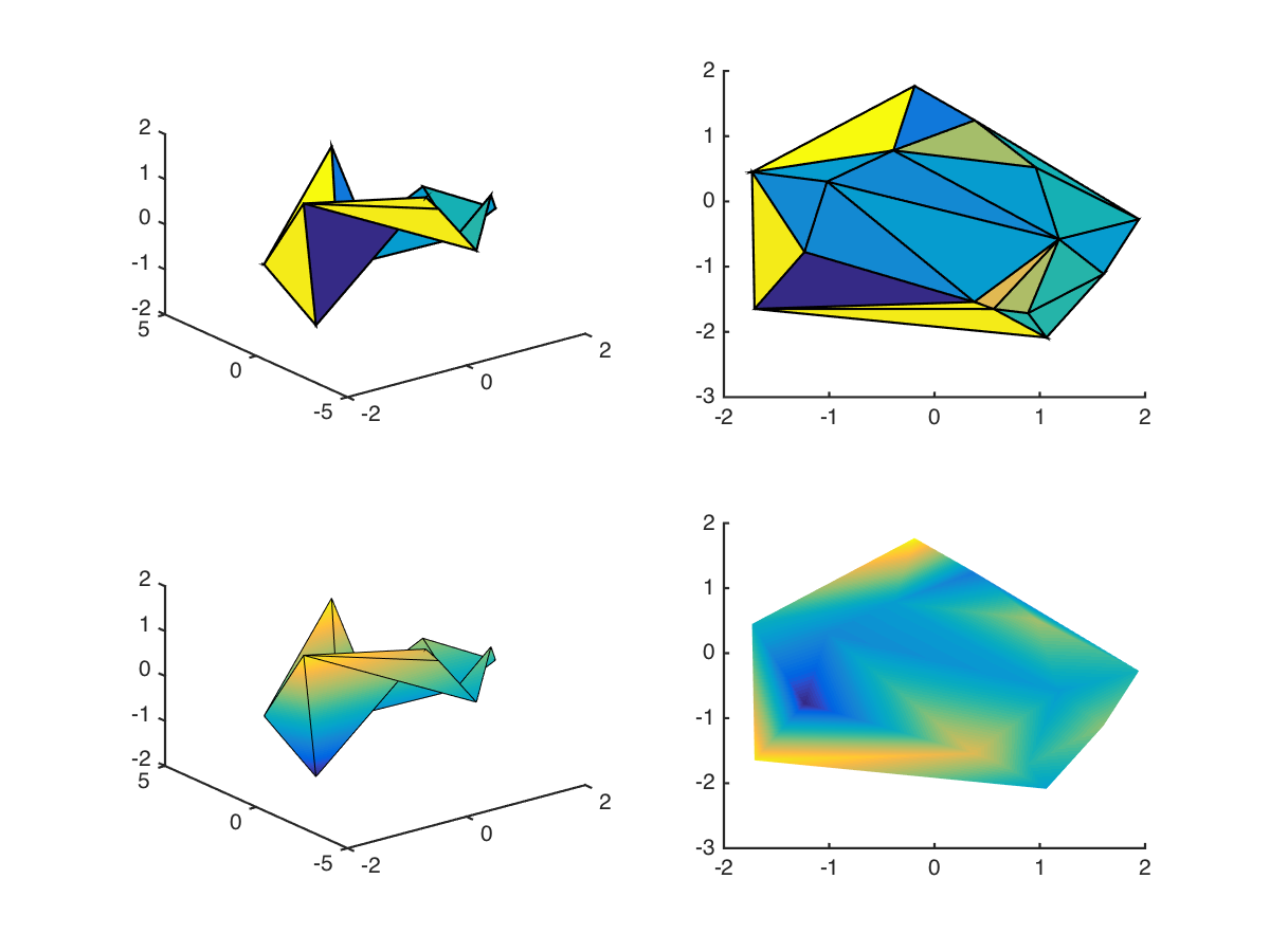
Note that without the interpolated shading, the plot is basically unusable. But even with interpolated shading, there’s significant distortion along certain diagonals. I’ve left out the edge lines in the bottom-right graph to emphasise this. If we resampled this function over a regular grid using scatteredInterpolant, we’d end up with points outside the original region, which might not always be appropriate. We could then delete the outsiders, but that would require additional processing. Wouldn’t it be nice to simply resample within the original?
Delaunay interpolation
To do this requires a couple steps. First, extract the Delaunay Triangularisation of our points:
DT = delaunay(x,y);
This function returns a list of 3xM indices into x and y, where M is the number of triangles. So if we extract the coordinates for each triangle and average them, we obtain the mid-point of each, including an interpolated value:
x2 = mean(x(DT),2);
y2 = mean(y(DT),2);
z2 = mean(z(DT),2);
This figure shows the grid that results after interpolating once and re-applying the Delaunay Triangularisation: (black before, red after)
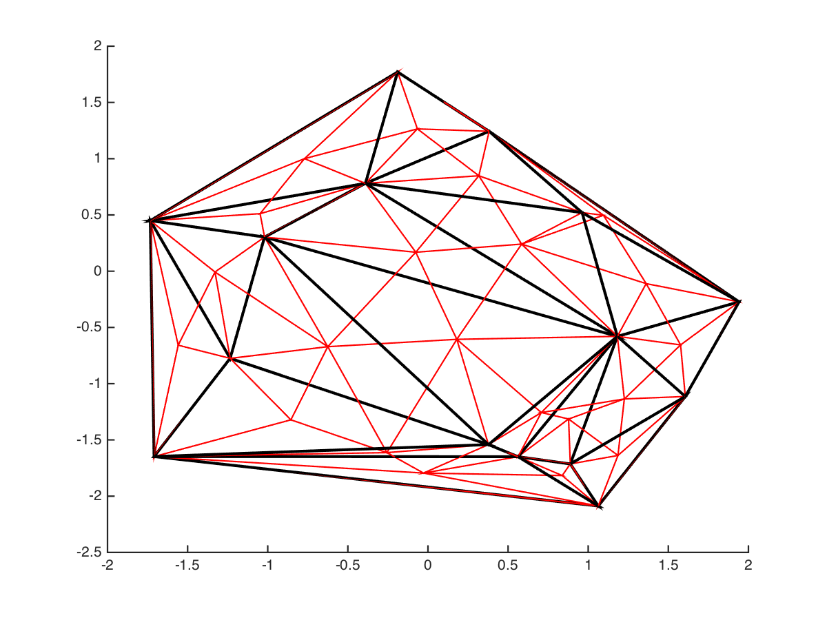
Note that the Delaunay algorithm doesn’t simply divide up the triangles into smaller components. We can then perform this iteratively to interpolate to an arbitrary level of detail:
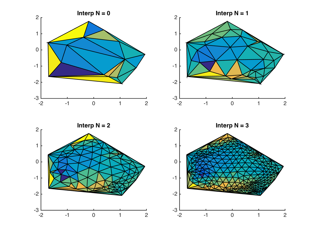
And after removing the grid lines and increasing the order, the results look pretty nice:
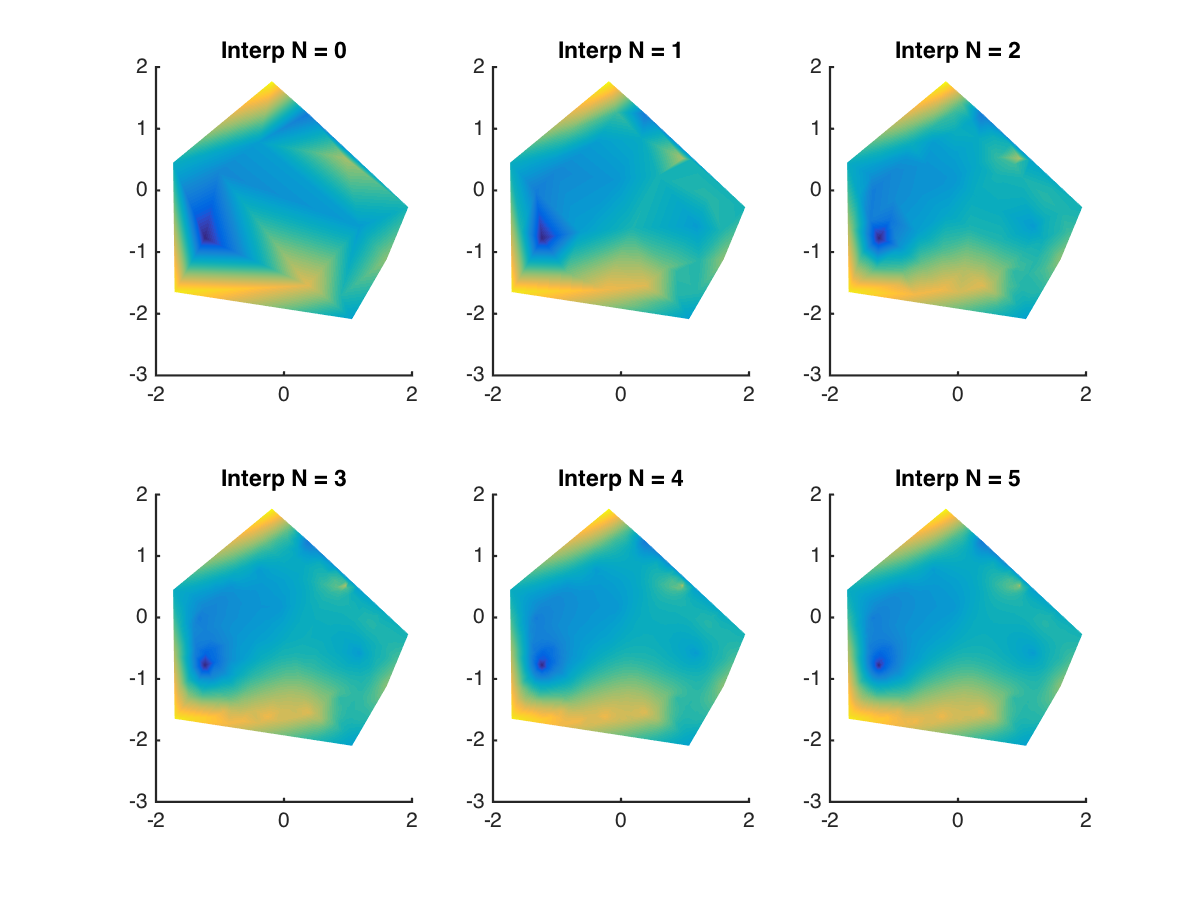
Interpolation will never solve the problem of under-sampling if there’s information missing, but it definitely helps to draw more pleasing figures.
I’ve uploaded this code to the Matlab file exchange under the name delaunay_surf, and added it to my generic Matlab repository on Github: https://github.com/wspr/matlabpkg. It’s pretty basic:
p = delaunay_surf(x,y,z,'N',4);
with a few additional options. Check out the example file for more, er, examples.
Happy plotting!