Smooth 3D curves in Matlab with John Hobby's algorithm
Drawing objects in Matlab is an excellent way of visualising the output of various mathematical routines, even if the end result is not intended to be graphical. In the early years of my PhD, I found visualisation an invaluable tool for checking code that required the movement and rotations of magnets in 3D space. I knew that the code ran, and actually showing the positions of the magnets used to generate various graphs was far more helpful that outputting coordinates for checking by hand, for example.
Matlab’s drawing and rendering methods are quite good but also somewhat limited. It’s possible to use quite sophisticated 3D rendering (e.g., Matlab skeleton); with a little work it’s possible to produce publication-ready graphics for which you might usually use a tool such as Asymptote.
Unfortunately, however, Matlab’s tools for creating graphics can be quite limited. Matlab provides commands to draw arrows, for example, but only in its ‘figure’ coordinate system so arrows cannot be drawn (without a great deal of work) to attach to points of interest in a graph (which are drawn in the ‘axis’ coordinate system). For this particular problem my colleague and partner in Matlab crime, Zebb Prime, has started to write some code that can draw nice arrows, even on curved lines.
But I digress. Another useful drawing tool that Matlab lacks is the ability to draw curved lines easily. (In fact, the Bezier curve routines I’m about to discuss are under-utilised in the modern world. Everyone that ever uses splines should know about Hobby’s work.) Bezier curves are usually specified in terms of key points and control points, where a smooth line connects the key points using the control points to specify curvature and tangential direction. I’m sure most people who have used Adobe Illustrator or similar vector drawing tools are quite familiar with this style of drawing curves. The maths behind it is all rather interesting, but when it comes down to actually doing the drawing, using control points is rather tedious, especially in a programmatic environment such as Matlab.
For this reason, John Hobby (1986) reformulated the Bezier curve maths such that it was parameterised in terms of logical variables such as tension and direction rather than control points.
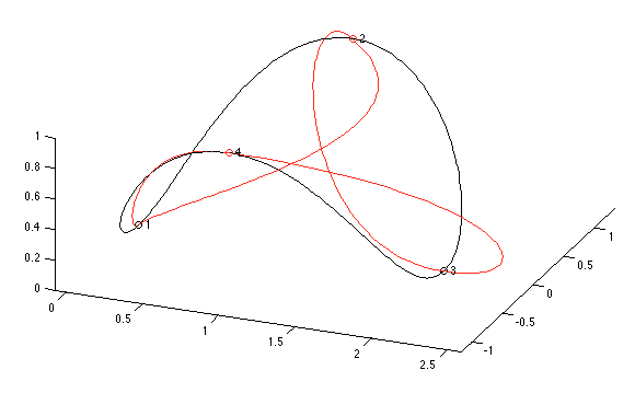
The huge advantage to his work is that complex curves can be drawn simply by specifying key points through which the curve must pass and the rest is calculated automatically. Here’s an example:

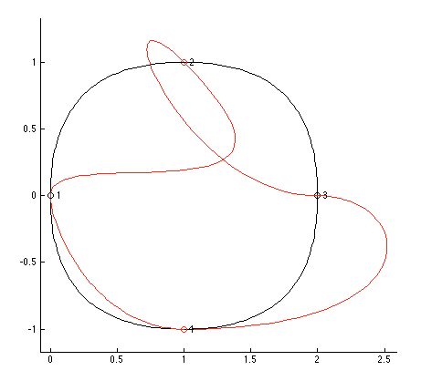
The key points specified are labelled one through four; the black curve shows how these four points connect with the default parameters, and the red curve shows what can be done by adjusting the directions that the curve must point when passing through two of the key points; a top view makes this quite clear:

And drawing these curves is as easy as something like (for the red curve):
points = {...
 [0 0 0],...
 {[1 1 1] [-1 1 0]},...
 {[2 0 0] [1 0 0]},...
 [1 -1 1]...
};
hobbysplines(points,'debug',true,'cycle',true,'color','red');
where the two explicit directions are given as unit vectors. For simplicity here I’ve omitted a couple of details for specifying tension.
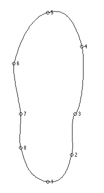
Once you are able to draw curves in this way, Matlab becomes much more useful as a general-purpose visualisation tool. Let’s say you wanted to visualise centre of pressure during an activity measured on a force platform. How would you draw the outline of a shoe in Matlab? I don’t know the best way, but selecting eight points and adjusting their positions makes it pretty easy:

(Don’t laugh at my ugly shoe. Obviously I’d spend some more time improving it if I actually needed it!)
Any discretised set of measurements can now be joined smoothly, but please don’t think of using this code to make a set of values into a smooth curve like you see all the time in Excel. You’re never allowed to do that!
You can download the code for drawing these curves from Github, where you can also send bugs or feature requests; the code will appear in the Matlab File Exchange shortly.